几何变换
几何变换
在阅读yolov3数据集处理图像增强代码时,发现了一段有意思的实现,写下博客记录下几种几何变换推导及利用opencv来可视化效果。
从网络上摘抄下仿射变换和透视变换来强化下印象:
仿射变换
仿射变换是二维坐标到二维坐标的线性变换,保持了二维图形的”平直性”(直线经过变换后仍是直线)和”平行性”(二维图形之间的相对位置关系保持不变,平行线依然是平行线,且直线上点的位置顺序不变)。任意的仿射变换都能表示为
[\begin{bmatrix}x’ \y’ \ 1\end{bmatrix}=\begin{bmatrix}m11& m12& m13 \ m21 & m22 & m23 \ 0 & 0 & 1 \end{bmatrix} \begin{bmatrix}x\y\1\end{bmatrix}]
从公示中可以看出有6个未知变量,可用不在同一条直线上的三个点来求出。
平移变换
平移变换可表示为
[\begin{bmatrix}x’ \y’ \ 1\end{bmatrix}=\begin{bmatrix}1& 0& m1 \ 0 & 1 & m2 \ 0 & 0 & 1 \end{bmatrix} \begin{bmatrix}x\y\1\end{bmatrix}]
该示例将图片中心平移到原点
import cv2
import numpy as np
import matplotlib.pyplot as plt

img = cv2.imread('demo.jpg')
h, w = img.shape[0], img.shape[1]

# translate
T = np.eye(3)
T[0, 2] = -img.shape[1] / 2
T[1, 2] = -img.shape[0] / 2

M = T
img2 = cv2.warpAffine(img, M[:2], dsize=(w, h), borderValue=(114, 114, 114))

ax = plt.subplots(1, 2, figsize=(12, 8))[1].ravel()
ax[0].imshow(img[:, :, ::-1])
ax[1].imshow(img2[:, :, ::-1])

plt.show()

旋转及缩放
opencv获取旋转矩阵的公示,简单的进行下推导,一般角度逆时针旋转为正,旋转角为θ,scale=s,示意图如图所示,设初始坐标点为(x, y),变换后的坐标点为(x’, y’),旋转及缩放变换可表示为
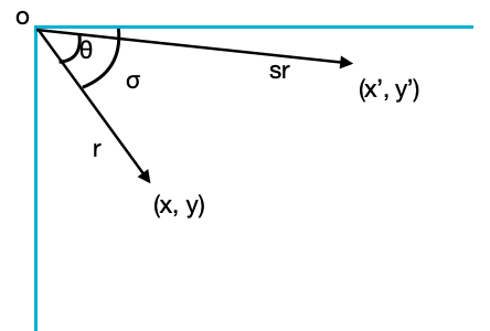
[x = rcos(\sigma)\ \ \ y = rsin(\sigma)]
[x’=srcos(\sigma-\theta)=srcos(\sigma)cos(\theta)+srsin(\sigma)sin(\theta)=xscos(\theta)+yssin(\theta)]
[y’=srsin(\sigma-\theta)=srsin(\sigma)cos(\theta)-srcos(\sigma)sin(\theta)=yscos(\theta)-xssin(\theta)]
假设绕指定点旋转(cx, cy),则可表示为平移+旋转缩放+平移,即
[\begin{bmatrix}x’ \y’ \ 1\end{bmatrix}=\begin{bmatrix}1& 0& cx \ 0 & 1 & cy \ 0 & 0 & 1 \end{bmatrix} \begin{bmatrix}scos(\theta)&ssin(\theta)&0 \-ssin(\theta)&scos(\theta)&0 \ 0&0&1 \end{bmatrix} \begin{bmatrix}1& 0& -cx \ 0 & 1 & -cy \ 0 & 0 & 1\end{bmatrix} \begin{bmatrix}x\y\1\end{bmatrix} = \begin{bmatrix}scos(\theta)&ssin(\theta)&(1-scos(\theta))cx - ssin(\theta)cy\-ssin(\theta)&scos(\theta)&ssin(\theta)cx+(1-scos(\theta))cy\0&0&1\end{bmatrix} \begin{bmatrix}x\y\1\end{bmatrix}]
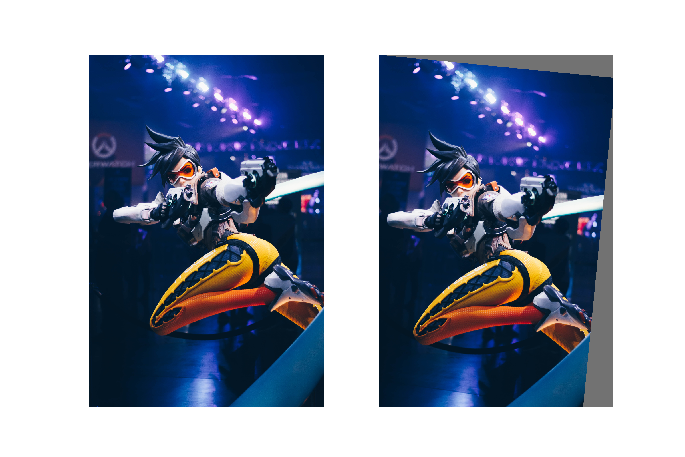
该示例为旋转缩放
import random
import math
import cv2
import numpy as np
import matplotlib.pyplot as plt

img = cv2.imread('demo.jpg')
h, w = img.shape[0], img.shape[1]

# rotation
degrees=10
scale = 0.1
R = np.eye(3)
a = random.uniform(-degrees, degrees)
s = random.uniform(1 - scale, 1 + scale)
R[:2] = cv2.getRotationMatrix2D(angle=a, center=(10, 10), scale=s)

M = R
img2 = cv2.warpAffine(img, M[:2], dsize=(w, h), borderValue=(114, 114, 114))
#img2 = cv2.warpPerspective(img, M, dsize=(w, h), borderValue=(114, 114, 114))

ax = plt.subplots(1, 2, figsize=(12, 8))[1].ravel()
ax[0].imshow(img[:, :, ::-1])
ax[1].imshow(img2[:, :, ::-1])
ax[0].axis('off')
ax[1].axis('off')
plt.show()
剪切变换
剪切变换可表示为
[\begin{bmatrix}x’ \y’ \ 1\end{bmatrix}=\begin{bmatrix}1& c& 0 \ d & 1 & 0 \ 0 & 0 & 1 \end{bmatrix} \begin{bmatrix}x\y\1\end{bmatrix}]
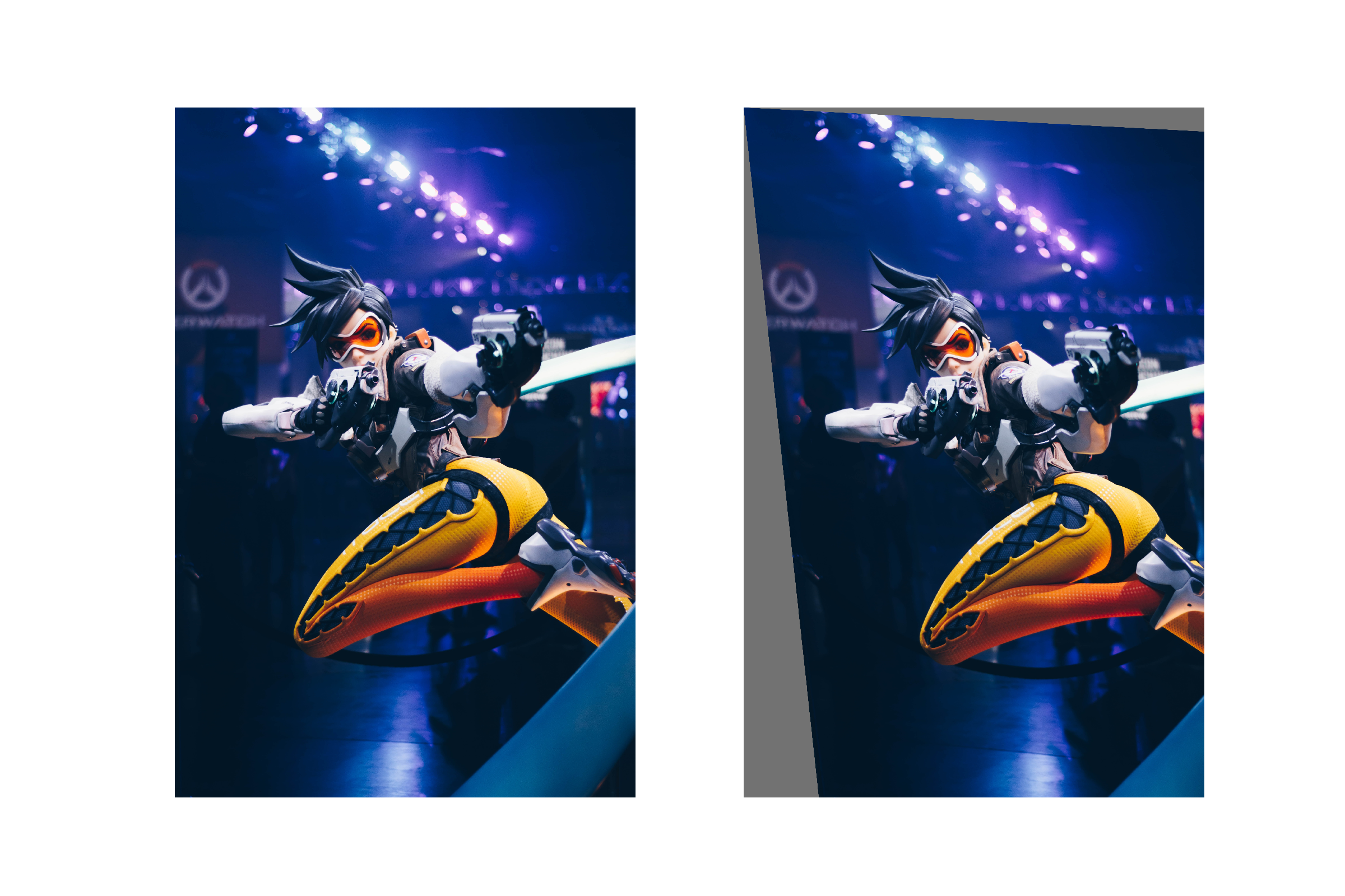
一个剪切变换的例子
import random
import math
import cv2
import numpy as np
import matplotlib.pyplot as plt

img = cv2.imread('demo.jpg')
h, w = img.shape[0], img.shape[1]

# shear
S = np.eye(3)
shear = 10
S[0, 1] = math.tanh(random.uniform(-shear, shear) * math.pi / 180)
S[1, 0] = math.tanh(random.uniform(-shear, shear) * math.pi / 180)

M = S
img2 = cv2.warpAffine(img, M[:2], dsize=(w, h), borderValue=(114, 114, 114))
#img2 = cv2.warpPerspective(img, M, dsize=(w, h), borderValue=(114, 114, 114))

ax = plt.subplots(1, 2, figsize=(12, 8))[1].ravel()
ax[0].imshow(img[:, :, ::-1])
ax[1].imshow(img2[:, :, ::-1])
ax[0].axis('off')
ax[1].axis('off')
plt.show()
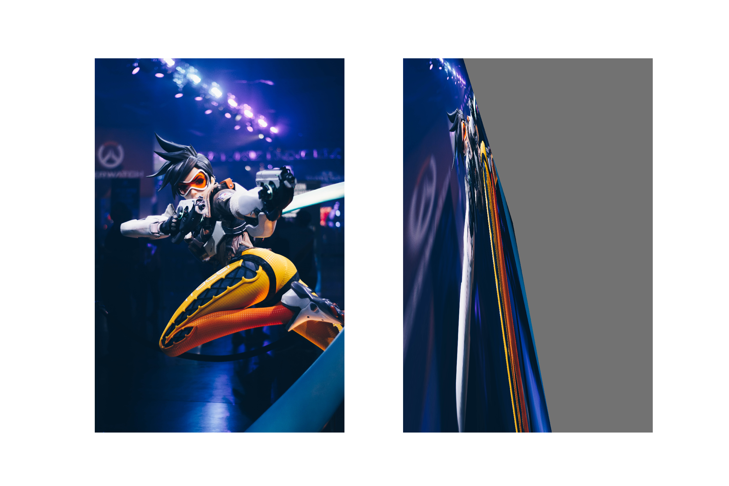
透视变换
透视变换是将图片投影到一个新的视平面,它是二维(x, y)到三维(X, Y, Z)再到另一个二维(x’, y’)的映射。相对于仿射变换,它将一个四边形区域映射到另一个四边形区域(不一定是平行四边形)。任意的透视变换都能表示为
[\begin{bmatrix}X \Y \ Z\end{bmatrix}=\begin{bmatrix}m11& m12& m13 \ m21 & m22 & m23 \ m31 & m32 & m33 \end{bmatrix} \begin{bmatrix}x\y\1\end{bmatrix}]
[x’=\frac{X}{Z} \ \ \ \ \ y’=\frac{Y}{Z}]
透视变换一般用于已知4组点,求解出变换矩阵M,在相机标定及双目视觉中较为常用。
一个简单的例子
import random
import math
import cv2
import numpy as np
import matplotlib.pyplot as plt

img = cv2.imread('demo.jpg')
h, w = img.shape[0], img.shape[1]

# translate
T = np.eye(3)
T[0, 2] = -img.shape[1] / 2
T[1, 2] = -img.shape[0] / 2

# rotation
degrees=10
scale = 0.1
R = np.eye(3)
a = random.uniform(-degrees, degrees)
s = random.uniform(1 - scale, 1 + scale)
R[:2] = cv2.getRotationMatrix2D(angle=a, center=(0, 0), scale=s)

# shear
S = np.eye(3)
shear = 10
S[0, 1] = math.tanh(random.uniform(-shear, shear) * math.pi / 180)
S[1, 0] = math.tanh(random.uniform(-shear, shear) * math.pi / 180)

# perspective
perspective = 0.001
P = np.eye(3)
P[2, 0] = random.uniform(-perspective, perspective)  # x perspective (about y)
P[2, 1] = random.uniform(-perspective, perspective)  # y perspective (about x)

#M = T @ S @ R @ P
M = P
#img2 = cv2.warpAffine(img, M[:2], dsize=(w, h), borderValue=(114, 114, 114))
img2 = cv2.warpPerspective(img, M, dsize=(w, h), borderValue=(114, 114, 114))

ax = plt.subplots(1, 2, figsize=(12, 8))[1].ravel()
ax[0].imshow(img[:, :, ::-1])
ax[1].imshow(img2[:, :, ::-1])
ax[0].axis('off')
ax[1].axis('off')
plt.show()
References
- https://blog.csdn.net/flyyufenfei/article/details/80208361